Rick Luettich 8/1/2025, rev 8/4/2026, rev 8/11/2026

1. Derivation

(adapted from J. Gao, 2018)

Consider that the radial profile of atmospheric pressure in a tropical cyclone can be expressed as a hyperbolic function of the deviation of the pressure from an ambient, far-field pressure Schloemer (1954), Holland (1980).

\[P(r) = P_{c} + \left( P_{n} - P_{c} \right)e^{- \frac{A}{r^{B_{g}}}}\tag{1}\]

\(P\)(\(r\)) is the atmospheric pressure (mb) at radius \(r\),\(\ P_{c}\) is the minimum central pressure (mb) in the eye of the cyclone, \(P_{n}\) is the ambient, far-field pressure, and \(e\) is the exponential function. \(A\) and \(B_{g}\) are scaling parameters.

Substituting this expression into the gradient wind balance in radial coordinates yields an equation for the tangential gradient wind at the top of the boundary layer:

\[V_{g}(r) = \sqrt{\frac{AB_{g}\left( P_{n} - P_{c} \right)e^{- \frac{A}{r^{B_{g}}}}}{\rho_{air}r^{B_{g}}} + \left( \frac{rf}{2} \right)^{2}} - \left( \frac{rf}{2} \right)\tag{2}\]

where \(V_{g}(r)\) is the gradient wind (m/s) at radius \(r\) (m) at the top of the boundary layer, \(\rho_{air}\) is the density of air (kg/m³), and \(f\) is the Coriolis parameter (s^-1).

Setting \(V_{g}\left( {r = R}_{mw} \right) = V_{\max}\), where \(R_{mw}\) (m) is the radius to maximum winds and \(V_{\max}\) (m/s) is the maximum wind speed at the top of the boundary layer, and rearranging terms, Eq (2) can be rewritten as:

\[\frac{AB_{g}\left( P_{n} - P_{c} \right)}{\rho_{air}} = e^{\frac{A}{{R_{mw}}^{B_{g}}}}{R_{mw}}^{B_{g}}\left\{ \left\lbrack V_{\max} + \ \left( \frac{R_{mw}f}{2} \right) \right\rbrack^{2} - \ \left( \frac{R_{mw}f}{2} \right)^{2} \right\}\tag{3}\]

Letting \(A \equiv \varphi\ {R_{mw}}^{B_{g}}\) and \(R_{o} \equiv \frac{V_{\max}}{R_{mw}f}\) and rearranging yields

\[\frac{AB_{g}\left( P_{n} - P_{c} \right)}{\rho_{air}} = e^{\varphi}{R_{mw}}^{B_{g}}\left\lbrack {V_{\max}}^{2}\left( 1 + {R_{o}}^{- 1} \right) \right\rbrack\tag{4}\]

substituting Eq (4) into Eq (2) yields:

\[V_{g}(r) = \sqrt{{V_{\max}}^{2}\left( 1 + {R_{o}}^{- 1} \right)\left( \frac{R_{mw}}{r} \right)^{B_{g}}e^{\varphi\left\lbrack 1 - \left( \frac{R_{mw}}{r} \right)^{B_{g}} \right\rbrack} + \left( \frac{rf}{2} \right)^{2}} - \left( \frac{rf}{2} \right)\tag{5}\]

A further constraint can be introduced by requiring that \(\frac{{dV}_{g}(r)}{dr} = 0\) at \(r = R_{mw}\). To differentiate Eq (5), first rearrange the equation as:

\[\left( V_{g}(r)\ + \frac{rf}{2} \right)^{2} = {V_{\max}}^{2}\left( 1 + {R_{o}}^{- 1} \right)\left( \frac{R_{mw}}{r} \right)^{B_{g}}e^{\varphi\left\lbrack 1 - \left( \frac{R_{mw}}{r} \right)^{B_{g}} \right\rbrack} + \left( \frac{rf}{2} \right)^{2}\]

Taking the derivatives of both sides (https://www.derivative-calculator.net):

\[2\left( V_{g}(r)\ + \frac{rf}{2} \right)\left( \frac{{dV}_{g}(r)}{dr} + \frac{f}{2} \right) = \frac{{V_{\max}}^{2}\left( 1 + {R_{o}}^{- 1} \right)B_{g}\left\lbrack \varphi\left( \frac{R_{mw}}{r} \right)^{B_{g}} - 1 \right\rbrack\left( \frac{R_{mw}}{r} \right)^{B_{g}}e^{\varphi\left\lbrack 1 - \left( \frac{R_{mw}}{r} \right)^{B_{g}} \right\rbrack}}{r} + \frac{rf^{2}}{2}\]

Setting \(\frac{{dV}_{g}(r)}{dr} = 0,\ V_{g}(r) = V_{\max}\ @\ r = R_{mw}\) yields:

\[V_{\max}f\ + \frac{R_{mw}f^{2}}{2} = \frac{{V_{\max}}^{2}\left( 1 + {R_{o}}^{- 1} \right)B_{g}\lbrack\varphi - 1\rbrack}{R_{mw}} + \frac{R_{mw}f^{2}}{2}\tag{6}\]

which can be easily simplified to:

\[R_{mw}f = V_{\max}\left( 1 + {R_{o}}^{- 1} \right)B_{g}\lbrack\varphi - 1\rbrack\ \ \ \ \ \ \ \ \ \ or\ \ \ \ \ \ \ \ \ \ \frac{1}{\left( 1 + R_{o} \right)} = B_{g}\lbrack\varphi - 1\rbrack\]

and therefore:

\[B_{g} = \frac{1}{\left( 1 + R_{o} \right)(\varphi - 1)}\ \ \ \ \ \ \ or\ \ \ \ \ \ \ \varphi = 1 + \frac{1}{B_{g}\left( 1 + R_{o} \right)}\tag{7}\]

Eliminating \(\varphi\), Eq. (4) can be re-written as:

\[B_{g} = e^{1 + \frac{1}{B_{g}\left( 1 + R_{o} \right)}}\frac{\left\lbrack {V_{\max}}^{2}\left( 1 + {R_{o}}^{- 1} \right) \right\rbrack}{\frac{\left( P_{n} - P_{c} \right)}{\rho_{air}}} - \frac{1}{\left( 1 + R_{o} \right)}\tag{8}\]

and Eq. (5) can be re-written as:

\[V_{g}(r) = \sqrt{{V_{\max}}^{2}\left( 1 + {R_{o}}^{- 1} \right)\left( \frac{R_{mw}}{r} \right)^{B_{g}}e^{\left( 1 + \frac{1}{B_{g}\left( 1 + R_{o} \right)} \right)\left\lbrack 1 - \left( \frac{R_{mw}}{r} \right)^{B_{g}} \right\rbrack} + \left( \frac{rf}{2} \right)^{2}} - \left( \frac{rf}{2} \right)\tag{9}\]

Rewriting \(R_{o}\)

\[R_{o} \equiv \frac{V_{\max}}{R_{mw}f} = \frac{V_{\max}}{rf}\frac{r}{R_{mw}} = \ R_{r}\ \frac{r}{R_{mw}} = \ R_{r}\ c^{- 1}\ \ \ where\ \ \ R_{r} \equiv \frac{V_{\max}}{rf}\ \ \ and\ \ \ \ c = \frac{R_{mw}}{r}\tag{10}\]

allows Eqs (8) and (9) to be written as:

\[B_{g} = e^{1 + \frac{1}{B_{g}\left( 1 + R_{r}c^{- 1} \right)}}\frac{\left\lbrack {V_{\max}}^{2}\left( 1 + c\ {R_{r}}^{- 1} \right) \right\rbrack}{\frac{\left( P_{n} - P_{c} \right)}{\rho_{air}}} - \frac{1}{\left( 1 + R_{r}c^{- 1} \right)}\tag{11}\] \[V_{g}(r) = \sqrt{{V_{\max}}^{2}\left( 1 + {cR_{r}}^{- 1} \right)c^{B_{g}}e^{\left( 1 + \frac{1}{B_{g}\left( 1 + R_{r}c^{- 1} \right)} \right)\left\lbrack 1 - c^{B_{g}} \right\rbrack} + \left( \frac{rf}{2} \right)^{2}} - \left( \frac{rf}{2} \right)\tag{12}\]

For given values of \(\frac{\left( P_{n} - P_{c} \right)}{\rho_{air}}\), \(V_{\max}\), and \(V_{g}(r)\), Eqs. (8) and (9) or alternatively Eqs (11) and (12) can be solved recursively to determine values of \(B_{g}\) and \(R_{mw}\). The latter equations involve only the unknowns \(B_{g}\) and \(c\), including the constraint that \(0 < c \leq 1\).

Finally, Eqs (8) and (11) can be written in terms of the original Holland (1980) \(B\) parameter,

\[B \equiv \ \frac{{V_{\max}}^{2}e}{\frac{\left( P_{n} - P_{c} \right)}{\rho_{air}}}\]

yielding:

\[B_{g} = Be^{\frac{1}{B_{g}\left( 1 + R_{o} \right)}}\left( 1 + {R_{o}}^{- 1} \right) - \frac{1}{\left( 1 + R_{o} \right)}\tag{13}\]

and

\[B_{g} = Be^{\frac{1}{B_{g}\left( 1 + R_{r}c^{- 1} \right)}}\left( 1 + c\ {R_{r}}^{- 1} \right) - \frac{1}{\left( 1 + R_{r}c^{- 1} \right)}\tag{14}\]

making it clear that \(B_{g} \rightarrow B\ \ \ as\ \ R_{o} = R_{r}\ c^{- 1}\ \rightarrow \ \infty\)

Dividing Eq (13) by B the resulting equation can be plotted, Figure 1:

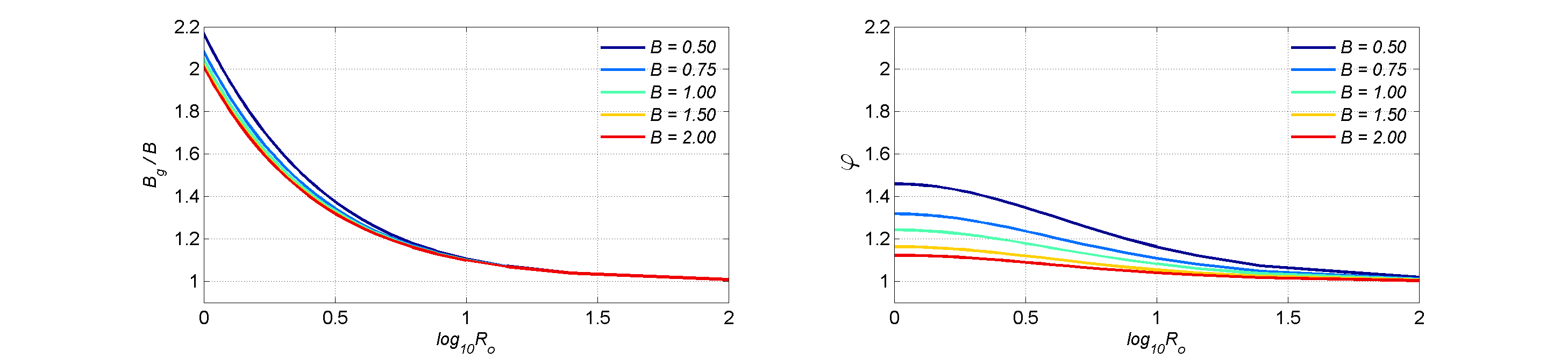
Figure 1. Profiles of \(\frac{B_{g}}{B}\) from GAHM with respect to \(\log_{10}R_{o}\) for different \(B\)values. (Figure 2.1 from Gao 2018).

Also, Eqs (9) and (12) can be written in a non-dimensional form:

\[\frac{V_{g}(r)}{V_{\max}} = \sqrt{\left( 1 + {R_{o}}^{- 1} \right)\left( \frac{R_{mw}}{r} \right)^{B_{g}}e^{\left( 1 + \frac{1}{B_{g}\left( 1 + R_{o} \right)} \right)\left\lbrack 1 - \left( \frac{R_{mw}}{r} \right)^{B_{g}} \right\rbrack} + \left( \frac{r}{R_{mw}} \right)^{2}\left( \frac{1}{{2R}_{o}} \right)^{2}} - \left( \frac{r}{R_{mw}} \right)\left( \frac{1}{{2R}_{o}} \right)\tag{15}\] \[\frac{V_{g}(r)}{V_{\max}} = \sqrt{\left( 1 + {cR_{r}}^{- 1} \right)c^{B_{g}}e^{\left( 1 + \frac{1}{B_{g}\left( 1 + R_{r}c^{- 1} \right)} \right)\left\lbrack 1 - c^{B_{g}} \right\rbrack} + \left( \frac{1}{{2R}_{r}} \right)^{2}} - \left( \frac{1}{{2R}_{r}} \right)\tag{16}\]

and plotted, Figure 2:

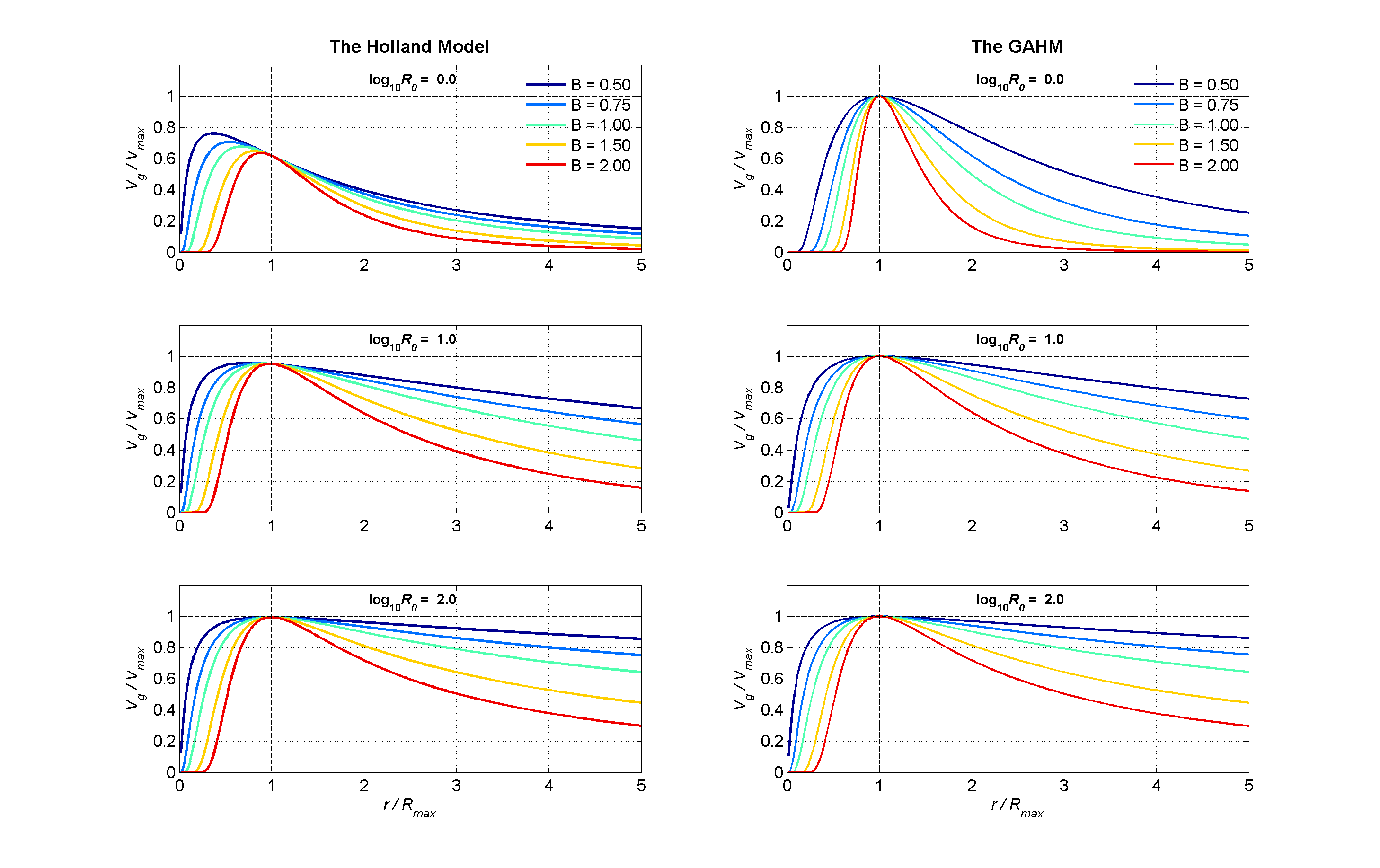
Figure 2. Normalized gradient wind profiles for the original Holland (1980) model and the GAHM for \(\log_{10}R_{o} = 0,\ 1,\ and\ 2\) (or correspondingly \(R_{o}\ = 1,\ 10,\ and\ 100\)) and B varying from 0.5 to 2. (Figure 2.3 from Gao 2018).

As a check, setting \(r = R_{mw}\) in Eq (15) yields

\[\frac{V_{g}(r)}{V_{\max}} = \sqrt{\left( 1 + {R_{o}}^{- 1} \right) + \left( \frac{1}{{2R}_{o}} \right)^{2}} - \left( \frac{1}{{2R}_{o}} \right)\] \[\frac{V_{g}(r)}{V_{\max}} = \frac{1}{2R_{o}}\sqrt{4R_{o}\left( R_{o} + 1 \right) + 1} - \left( \frac{1}{{2R}_{o}} \right)\] \[\frac{V_{g}(r)}{V_{\max}} = \frac{1}{2R_{o}}\sqrt{\left( 2R_{o} + 1 \right)^{2}} - \left( \frac{1}{{2R}_{o}} \right) = 1\]

It is helpful to use GAHM to compute the pressure deficit, from Eq (1).

\[P(r) - P_{n}\ = \left( P_{n} - P_{c} \right)\left( e^{- \frac{A}{r^{B_{g}}}} - 1 \right) = \left( P_{n} - P_{c} \right)\left( e^{- {\varphi\left( \frac{R_{mw}}{r} \right)}^{B_{g}}} - 1 \right)\tag{17}\]

2. Implementation

Data requirements for GAHM2026 are comprised of values for the eye position (lon, lat), the minimum total central pressure (mb), \(P_{c}\), the ambient pressure (mb), \(P_{n}\), the 1-min sustained maximum total wind speed at 10m height above ground (kt), \(V_{max\_ 1\_ 10}\), and the radial distances (nautical miles) from the TC eye to the 1-min sustained, 64, 50, and 34 knot total wind speed isotachs in the NE, SE, SW, and NW quadrants. Total pressure and total wind speed refer to the sum of the vortex and large-scale environmental fields a TC is experiencing. In the latter case the total wind speed is the magnitude of the vector sum of the vortex wind velocity and the large-scale environmental wind velocity. The ambient pressure is derived from the large-scale environmental pressure field, although in ADCIRC it is assumed to have a fixed value of 1013 mb. The radius of maximum winds (nautical miles), \(R_{mw}\), may be used by GAHM2026 as a default value if other values are missing or inconsistent.

It is assumed that \(V_{g}(r),\ \ V_{\max}\) in the previous section represent 10 min average vortex speeds at the top of the boundary layer (and thus above the influence of friction with the land/water surface) whose directions are oriented perpendicular to a radial line from the eye location, (i.e., locally tangent to the storm vortex). These are designated \(V_{vor\_ 10\_ tbl},\ \ V_{max\_ vor\_ 10\_ tbl}\) where the \(vor\) subscript denotes “vortex field”, the initial _10 subscript denotes 10-min average, and the latter _tbl subscript denotes a height equal to the top of the boundary layer.

It is assumed that the input pressure values, \(P_{c}\) , \(P_{n}\)are 10-min averages and the pressure deficit, \(P_{n} - \ P_{c}\), is equivalent at 10 m height and at the top of the boundary layer.

GAHM2026 is implemented as a two-step process. Initially, track file values including the isotach distances are used with Eqs (9) or (12) to compute \(B_{g}\ and\ R_{mw}\)for each quadrant. Once computed, these and the track file values are used to compute the radial velocity and pressure profiles at the central angle of each quadrant. The radial profiles are interpolated azimuthally to create radial profiles at a specified angular increment. If blending with a large-scale field is specified, the blending is done for each radial profile. As a final step the radial profiles are interpolated to a regular grid that is centered on the eye of the storm.

The remaining paragraphs in this section provide the details of the calculation of quadrant values of \(B_{g}\ and\ R_{mw}\).

Convert 1-min sustained wind speeds to 10-min averaged values: It is assumed that the maximum total wind speed and the 64, 50 and 34 knot isotach input wind speeds must be converted from 1-min sustained values to 10-min averaged values using a conversion factor one2ten = 0.89 (e.g., Kruk et al, 2010), i.e.,

\[V_{max\_ 10\_ 10} = \ {one2ten*V}_{max\_ 1\_ 10}\]

(A similar factor of 0.88 is recommended to convert 1-min to 10-min sustained values, IBTrACS 2025). The factor one2ten is specified in the GAHM2026 configuration file.

Convert 10 m above ground to the top of the boundary layer values: It is assumed that all wind velocities at the top of the boundary layer and 10 m above ground are related via a boundary layer factor, BLF, i.e.,

\[V_{\_ 10\_ 10} = \ {BLF*V}_{\_ 10\_ tbl}\]

and that moving from the top of the boundary layer to 10-m height, in the northern (southern) hemisphere, the vortex component of the velocity experiences a counterclockwise (clockwise) turning angle defined as:

Turning angle (deg) \({= 10*r/R}_{mw}\ \ \ \ \ \ \ \ \ \ \ \ \ \ \ \ \ \ \ \ \ \ \ \ \ \ \ if\ r \leq R_{mw}\)

Turning angle (deg) \({= 10 + 75*(r/R}_{mw} - 1)\ \ \ \ \ if\ R_{mw} < r \leq 1.2*R_{mw}\)

Turning angle (deg) \(= 25\ \ \ \ \ \ \ \ \ \ \ \ \ \ \ \ \ \ \ \ \ \ \ \ \ \ \ \ \ \ \ \ \ \ \ \ \ \ \ \ \ \ \ \ \ if\ 1.2*R_{mw} < r\)

Multiple studies have analyzed the reduction of wind speed between flight level (typically 700-hPa) and the surface (10 m) with a reduction factor of 0.9 often cited, e.g., Franklin et al (2003). However, the 700-hPa level is typically significantly higher than the top of the frictional boundary layer and the 700-hPa wind speed is often less than that at the top of the boundary layer, particularly near the core of the storm, suggesting a \({BLF\sim 0.8 - 0.9}_{}\) in this region. This is less the case outside of the \(R_{mw}\) and therefore a value of \({BLF \approx 0.9}_{}\) may be more appropriate in this region. Note, GAHM2026 uses a space and time constant \(BLF\) that is specified in the GAHM2026 configuration file. A value \(BLF = 0.9\) is commonly used.

Decompose the total pressure field and total wind velocity field into "vortex fields" and "environmental fields": As noted above, it is assumed that the input wind and pressure fields are total fields that represent the sums of “vortex fields”, \(P_{c\_ vor\_ 10\_ 10},V_{vor\_ 1\_ 10}\), and “environmental fields”, \(P_{c\_ env\_ 10\_ 10},V_{env\_ 10\_ 10}\), reflecting larger scale spatial processes. Due to the linear scaling between 10 m elevation and the top of the boundary layer, this separation is applicable either at a height of 10 m above ground, i.e., \(V_{\_ 10\_ 10} = \ V_{vor\_ 10\_ 10} + \ V_{env\_ 10\_ 10}\), or at the top of the boundary layer, i.e., \(V_{\_ 10\_ tbl} = \ V_{vor\_ 10\_ tbl} + \ V_{env\_ 10\_ tbl}\), as long as the turning angle is accounted for.

The “environmental fields”, \(P_{c\_ env\_ 10\_ 10},V_{env\_ 10\_ 10}\), may either be inferred from the storm’s translation velocity, \(V_{trans}\) or extracted from large scale gridded model data. GAHM2026 supports three options:

a. ADCIRC assumes \(V_{env\_ 1\_ 10\ } = 1.5*\ {V_{trans}}^{0.63}\) (for \(V_{trans}\) in knots) or \(V_{env\_ 1\_ 10\ } = 1.5*\ {V_{trans}}^{0.63}*{0.51444}^{0.37}\) (for \(V_{trans}\) in m/s) and \(V_{env\_ 1\_ 10\ }\) varies with radial distance from the eye following the same relationship as \(V_{g}(r)\), Eq. (9) or (12). Once computed, one2ten is used to convert the 1-min sustained to a 10-min average value as described above. GAHM2026 offers a similar option, however, it is assumed that the resulting environmental velocity better reflects 10-min averaged value than a 1-min sustained value and therefore that \(V_{env\_ 10\_ 10\ } = 1.5*\ {V_{trans}}^{0.63}\) or \(V_{env\_ 10\_ 10\ } = 1.5*\ {V_{trans}}^{0.63}*{0.51444}^{0.37}\). The resulting environmental fields vary in time and vary radially in space.

b. Lin and Chavas (2012) analyzed H*Wind snapshots and concluded that a spatially constant \(V_{env\_ xx\_ 10\ } = 0.55*V_{trans}\) where \(V_{env\_ xx\_ 10}\) is rotated 20 degrees counterclockwise from \(V_{trans}\), is better supported than the value assumed in ADCIRC. In GAHM2026 this option is implemented assuming that \(V_{env\_ 10\_ 10\ } = 0.6*V_{trans}\) where \(V_{env\_ 10\_ 10}\) is rotated 20 degrees counterclockwise from \(V_{trans}\). The 0.6 multiplier follows Wang et al (2021). The resulting environmental fields vary in time but are spatially constant.

c. GAHM2026 can also extract spatially varying environmental fields from large scale gridded wind and pressure fields such as ERA5. A 5^th order Butterworth digital filter to low pass filter the fields to obtain \(P_{c\_ env\_ 10\_ 10},V_{env\_ 10\_ 10}\). This is commonly used when the resulting vortex will be blended back into the large-scale field, but can also be used without blending and produces environmental fields that vary in space and time.

The following steps are required to implement these features.

1. Compute the 10-min averaged, maximum vortex velocity at the top of the boundary layer. Initially the maximum vortex velocity at 10 m elevation, \(V_{\max\_ vor\_ 10\_ 10},\) is determined from the input total maximum velocity magnitude, \(\left\vert V_{max\_ 1\_ 10\ } \right\vert\) and the environmental velocity, \(V_{env\_ 10\_ 10\ }\). The total maximum velocity occurs where the environmental velocity and the maximum vortex velocity are aligned, i.e.,

\[V_{max\_ 10\_ 10} = one2ten*\left\vert V_{\max\_ 1\_ 10} \right\vert \ *V_{envuv\_ 10\_ 10}\]

where \(V_{envuv\_ 10\_ 10}\) is the unit vector in the direction of \(V_{env\_ 10\_ 10}\). Because of this alignment, the magnitude of the maximum, tangential vortex velocity is equal to the difference between the magnitudes of the input total maximum velocity and the environmental velocity.

\[\left\vert V_{\max\_ vor\_ 10\_ 10} \right\vert = \left\vert V_{\max\_ 10\_ 10} \right\vert - \ \left\vert V_{env\_ 10\_ 10} \right\vert\]

The maximum vortex velocity at the top of the boundary layer is thus equal to

\[V_{max\_ vor\_ 10\_ tbl} = \ \left( \frac{\left\vert V_{\max\_ vor\_ 10\_ 10} \right\vert }{BLF} \right)*V_{voruv\_ tbl}\]

where the vortex velocity unit vector at the top of the boundary layer, \(V_{voruv\_ tbl}\), is perpendicular to a radial line from the vortex eye and directed ccw in the northern hemisphere (cw in the southern hemisphere) at any location. The location around the vortex where \(V_{\max\_ vor\_ 10\_ 10}\) occurs is determined by the direction of the environmental velocity at 10 m. The location around the vortex where \(V_{\max\_ vor\_ 10\_ tbl}\) occurs is adjusted from the 10 m height by the vortex turning angle.

Once an initial estimate is obtained for \(\left\vert V_{\max\_ vor\_ 10\_ tbl} \right\vert\) , this should be checked to ensure that it is greater than a specified minimum value, \(\left\vert V_{\max vor\_ 10\_ tbl} \right\vert _{\min}\). If this condition is violated, GAHM should not be used. Note, \(\left\vert V_{\max vor\_ 10\_ tbl} \right\vert _{\min}\) is specified in the GAHM2026 configuration file. A default value of 20 kts is suggested.

2. Assuming the availability of isotach total wind magnitudes (i.e., \(\left\vert {VQuad}_{\_ 1\_ 10} \right\vert =\)64, 50, 34 kts at specified radial distances from the eye in the NE, SE, SW and NW quadrants), these need to be converted to 10-min, vortex velocities at the top of the boundary layer, \({VQuad}_{vor\_ 10\_ tbl}\). These are written as:

\[{VQuad}_{vor\_ 10\_ tbl} = \ \left\vert {VQuad}_{vor\_ 10\_ tbl} \right\vert *\ {VQuad}_{voruv\_ tbl}\]

where the unit vector in each quadrant, \({VQuad}_{voruv\_ tbl}\), is assumed to be perpendicular to a radial line from the vortex eye to the midpoint of the quadrant arc and directed counterclockwise (clockwise) in the northern (southern) hemisphere. For example, in the northern hemisphere the unit vector for the NE quadrant would point NW (315 deg clockwise from North). Given this, the quadrant vortex velocity at 10 m height is:

\[{VQuad}_{vor\_ 10\_ 10} = \ BLF*\left\vert {VQuad}_{vor\_ 10\_ tbl} \right\vert *{VQuad}_{voruv\_ 10}\]

where the quadrant unit vector at 10 m, \({VQuad}_{voruv\_ 10}\), is equal to the value at the top of the boundary layer adjusted for the vortex turning angle.

Assuming the isotach value represents the magnitude of the total wind velocity, this can be expressed as the magnitude of the sum of the vortex and environmental components,

\[one2ten*\left\vert {VQuad}_{\_ 1\_ 10} \right\vert = \left\vert {VQuad}_{\_ 10\_ 10} \right\vert = \ \left\vert {VQuad}_{vor\_ 10\_ 10} + \ V_{env\_ 10\_ 10} \right\vert\]

which can be solved for the unknown \(\left\vert {VQuad}_{vor\_ 10\_ 10} \right\vert\).

Two consistency checks are performed to ensure this relationship can yield a physically valid solution.

a. The first check assumes that fitting the gradient wind balance to the isotach is valid only if \(\left\vert {VQuad}_{vor\_ 10\_ tbl} \right\vert \geq \left\vert {VQuad}_{vor\_ 10\_ tbl} \right\vert _{\min}\). Setting \(\left\vert {VQuad}_{vor\_ 10\_ tbl} \right\vert = \left\vert {VQuad}_{vor\_ 10\_ tbl} \right\vert _{\min}\) , the above equation can be evaluated to determine a minimum acceptable value of \(\left\vert {VQuad}_{1\_ 10} \right\vert _{\min}\). If \(\left\vert {VQuad}_{1\_ 10} \right\vert {< \left\vert {VQuad}_{1\_ 10} \right\vert }_{\min}\), the isotach should not be used to determine \(R_{mw}\), and rather \(R_{mw}\) is determined from the next higher isotach in the quadrant. A reasonable value for \(\left\vert {VQuad}_{vor\_ 10\_ tbl} \right\vert _{\min}\) is assumed to be 5 kts. This value is specified in the GAHM2026 configuration file.

b. The second check assumes that \(\left\vert {VQuad}_{vor\_ 10\_ tbl} \right\vert \leq \left\vert V_{\max\_ vor\_ 10\_ tbl} \right\vert\). Setting \(\left\vert {VQuad}_{vor\_ 10\_ tbl} \right\vert = \left\vert V_{max\_ vor\_ 10\_ tbl} \right\vert\), the above equation can be evaluated to determine a maximum acceptable value of \(\left\vert {VQuad}_{1\_ 10} \right\vert _{\max}\). If this is violated, the isotach should not be used to determine \(R_{mw}\), and rather \(R_{mw}\) is determined from the next higher isotach in the quadrant and \(\left\vert {VQuad}_{vor\_ 10\_ tbl} \right\vert = \left\vert V_{\max\_ vor\_ 10\_ tbl} \right\vert\).

If both conditions are satisfied, \(\left\vert {VQuad}_{vor\_ 10\_ 10} \right\vert\) is solved by squaring both sides and expanding the right-hand side to yield:

\[\left\vert {VQuad}_{vor\_ 10\_ 10} \right\vert ^{2} + 2\left\vert {VQuad}_{vor\_ 10\_ 10} \right\vert \left\vert V_{env\_ 10\_ 10} \right\vert \left( {VQuad}_{voruv\_ 10\_ 10}\ \bullet V_{envuv\_ 10\_ 10} \right)\] \[+ \left\vert V_{env\_ 10\_ 10} \right\vert ^{2} - \left\vert {VQuad}_{\_ 10\_ 10} \right\vert ^{2} = 0\]

which can be solved for \(\left\vert {VQuad}_{vor\_ 10\_ 10} \right\vert\) using the quadratic formula.

For the environmental field implemented in ADCIRC, the radial profile of \(\left\vert V_{env\_ 10\_ 10} \right\vert\) is assumed to match the radial profile of the vortex gradient wind, i.e.,

\[\left\vert V_{env\_ 10\_ 10} \right\vert = \ \left\vert {V^{*}}_{env\_ 10\_ 10} \right\vert *\frac{\left\vert {VQuad}_{vor\_ 10\_ 10} \right\vert }{\left\vert V_{max\_ vor\_ 10\_ 10} \right\vert }\]

where \({V^{*}}_{env\_ 10\_ 10}\) is the environmental velocity at \(r = R_{mw}\). In this case the quadratic equation simplifies to:

\[\left\vert {VQuad}_{vor\_ 10\_ 10} \right\vert \ = \frac{\left\vert {VQuad}_{\_ 10\_ 10} \right\vert }{\left\vert {VQuad}_{voruv\_ 10\_ 10} + V_{envuv\_ 10\_ 10}\frac{\left\vert {V^{*}}_{env\_ 10\_ 10} \right\vert }{\left\vert {VMax}_{vor\_ 10\_ 10} \right\vert } \right\vert }\]

3. GAHM2026 default conditions / assumptions

The following are checked / set in GAHM2026_consistency.m

If no isotach distances exist in a quadrant, \(R_{mw}\) for that quadrant is determined as the average value from the quadrant(s) having valid values. \(B_{g}\) is determined from Eq. (13).

Depending on the outcome of the following diagnostic checks, flags are set and used to set default conditions. These are available for output to clarify whether default values were used. The isotach indices i=1:4 correspond to 1=34kt, 2=50kt, 3=64kt, 4=00kt. The quadrant indices q=1:4 correspond to NE, SE, SW, NW. The first index is the quadrant index and the second is the isotach index.

1. Check whether Holland 1980 B value falls within specified limits

If Bmin <= B <= Bmax GAHM.flag_B=1

if B < Bmin B is reset = Bmin, GAHM.flag_B=0

if B > Bmax, B is reset = Bmax, GAHM.flag_B=2

Note: Bmin, Bmax are specified in the GAHM2026 configuration file. Suggested values are 0.5 and 2.5.

2. Check if any isotach (34kt, 50kt, 64kt) distances are present in any quadrant in the track file for the current time. If none are present, GAHM.flag(1:4,1:4) = 0. \(R_{mw}\) in all quadrants = \(R_{mw}\) read in from the track file. \(B_{g}\), (A, phi) are computed from GAHM2026.

3. Check that \(\left\vert V_{\max\_ vor\_ 10\_ tbl} \right\vert \geq \left\vert V_{\max vor\_ 10\_ tbl} \right\vert _{\min}\) - this ensures that the vortex maximum speed at the top of the boundary layer, is strong enough (e.g., >20 kts) to use the GAHM gradient wind balance to compute \(R_{mw}\). \(\left\vert V_{\max vor\_ 10\_ tbl} \right\vert _{\min}\) is set in the GAHM2026 configuration file. If this condition is not met, GAHM.flag(1:4,1:3)=2, GAHM.flag(1:4,4)=0, \(R_{mw}\) in all quadrants = \(R_{mw}\) read in from the track file. \(B_{g}\), (A, phi) are computed from GAHM2026.

4. Check if an isotach distance is present in the track file for a specific quadrant, isotach pair. If not, GAHM.flag(q,i)=0;

5. Check that \(\left\vert {VQuad}_{vor\_ 10\_ tbl} \right\vert \geq \left\vert {VQuad}_{vor\_ 10\_ tbl} \right\vert _{\min}\) - this ensures that the vortex isotach speed in each quadrant at the top of the boundary layer is strong enough (e.g., 5 kts) to use GAHM gradient wind balance to compute \(R_{mw}\). \(\left\vert {VQuad}_{vor\_ 10\_ tbl} \right\vert _{\min}\)is set in the GAHM2026 configuration file. This is checked for each quadrant, isotach pair. If this condition is not met, then GAHM_flag(q,i)=3. \(R_{mw}\) is copied from surrounding isotachs (e.g., next higher isotach in quadrant). \(B_{g}\), (A, phi) are computed from GAHM2026.

6. Check that \(\left\vert V_{\max\_ vor\_ 10\_ 10} \right\vert \geq \left\vert {VQuad}_{vor\_ 10\_ 10}\ (q,i) \right\vert\) - this ensures that the vortex isotach speeds in each quadrant are < or = the vortex maximum speeded. This is checked for each (quadrant, isotach) pair assuming 10 and 25 deg ccw turning angles from the top of the boundary layer to 10m. If this condition is not met for both turning angles, GAHM_flag(q,i)=4. In this case assume \(R_{mw}\)= is copied from the highest available isotach value in the quadrant(?), \(\left\vert {VQuad}_{vor\_ 10\_ 10}\ (q,i) \right\vert = \left\vert V_{\max\_ vor\_ 10\_ 10} \right\vert\), \(B_{g}\), (A, phi) are computed from GAHM2026. If the condition is not met for only one of the turning angles, GAHM_flag(q,i)=5. An intermediate turning angle is estimated and use to determine \(R_{mw}\), \(B_{g}\), (A, phi) are computed from GAHM2026.

4. Blending with gridded large-scale fields

GAHM2026 can generate either standalone tropical cyclone (TC) wind and pressure fields or TC fields that are blended with gridded large-scale fields (e.g., ERA5). As discussed in the previous section, GAHM2026 TC fields are comprised of the sum of TC vortex (from the GAHM equations) and environmental fields. If blending is desired, the environmental fields are computed by spatially low pass filtering the gridded large-scale fields to remove their TC vortex component.

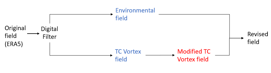
Figure 1. General schematic of the blending strategy

A 5^th order Butterworth digital filter with half power set at a length scale that is 25 times the average radius to the 10 kt isotach in the gridded large-scale field is applied in the meridional and zonal directions.

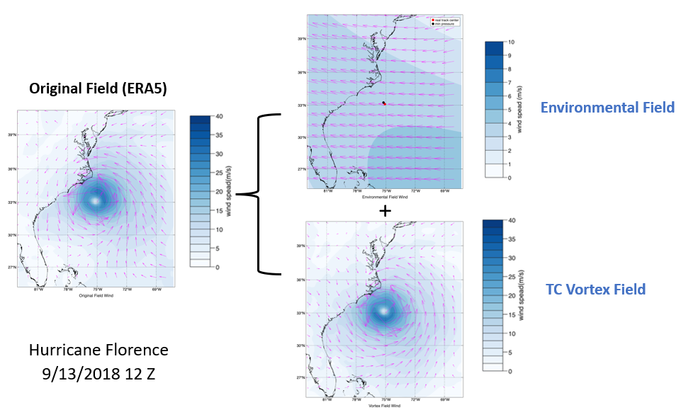
Figure 2. Example of separated environmental and TC vortex fields from gridded ERA5 fields for Hurricane Florence

The GAHM TC vortex field is then blended into the original TC vortex field along radial lines from the TC eye using a hyperbolic tangent smoothing function between the two radial distances r1 and r2:

taper = 1 r<=r1

taper = 0.5*(1 + tanh(a*(1-2*(r-r1)/(r2-r1)))/tanh(a))

taper = 0 r>r2

a, r1, and r2 are specified in the GAHM2026 configuration file. The “a” parameter controls the shape of the hyperbolic tangent function; a=1 yields a nearly linear taper between r1 and r2; a > 1 yields a more s-shaped taper between r1 and r2. Typical values are a=2, r1 = distance to the 34 kt isotach, r2 = distance to the 20 kt isotach.

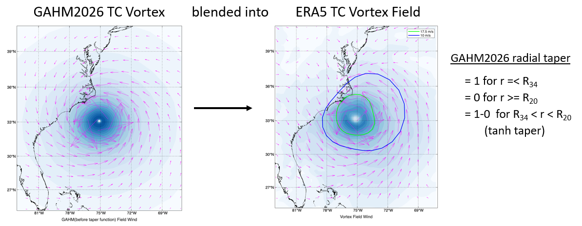
Figure 3. Example of GAHM2026 TC vortex to be blended into the ERA5 TC vortex field. The green and blue lines represent the 34 kt and 20 kt isotachs, respectively.

The modified (blended) TC vortex field is then added back to the environmental field to yield the final blended result.

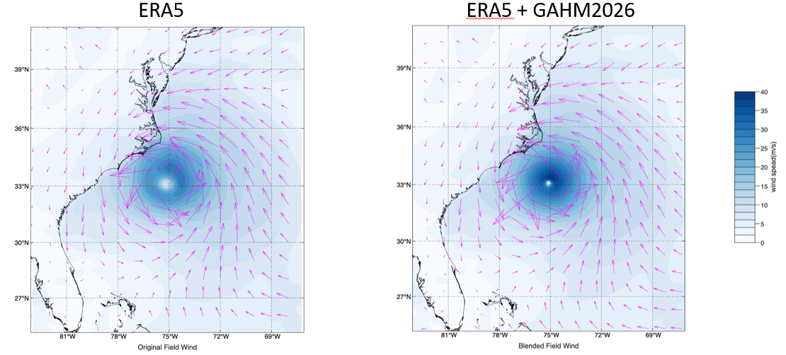
Figure 4. Example of the original ERA5 wind field representation of Hurricane Florence and the revised wind field representation after blending in the GAHM2026 TC vortex.

5. Wind Adjustment Factor (WAF)

GAHM2026 can modify wind speeds to account for the reduction that occurs when wind moves from marine roughness to land roughness. This has been implemented using a wind reduction algorithm (Simiu and Scanlan 1986) similar to that implemented in ADCIRC.

Wind Speed_land = WAF * Wind Speed_marine

WAF = (Zo_land /Zo_marine)^0.0706 *ln(10/Zo_land)/ln(10/Zo_marine)

where Zo_land and Zo_marine are effective roughnesses in the upwind direction. The WAF is precomputed either on a grid or at specified points based on land cover data, e.g., as found in the National Land Cover Database (NLCD) or the Coastal Change Analysis Program Land Cover database (C-CAP), Figure 5.

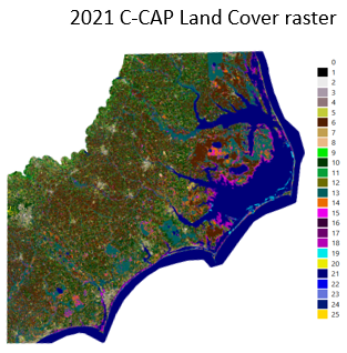
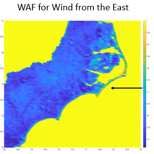
Figure 5. C-CAP land cover raster and classification categories for eastern North Carolina and resulting WAF for a wind blowing from due East.

Land cover types are converted to roughness values and Zo_land is computed as a weighted average over up wind sectors using a gaussian weighting that decays with distance from the adjustment location (Westerink et al, 2008), Figure 6. Zo_marine = 0.001 m is assumed.

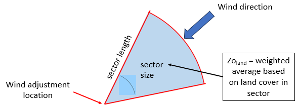
Figure 6. Schematic of the calculation of the effective roughness

WAF is precomputed in a specified number of upwind directions and sector properties. GAHM2026 interpolates between the precomputed values based on the location and wind direction. WAF has the effect of reducing the wind speed over land and creating over water shadow zones in areas where the wind is blowing from land to water, Figure 7, 8.

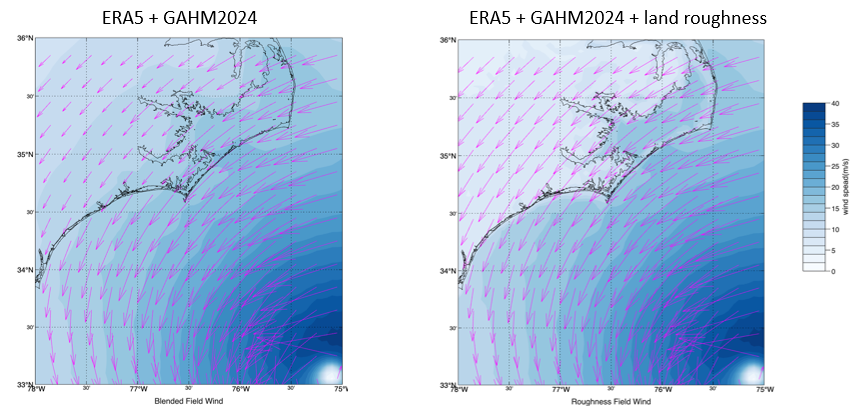
Figure 7. Example of blended ERA5 + GAHM2026 wind speed with and without WAF

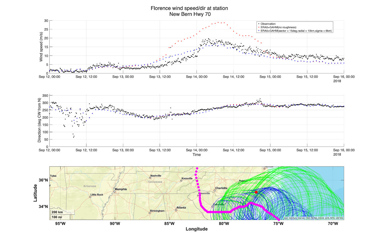
Figure 8. Comparison of observational data and blended ERA5+GAHM2026 wind speed with and without WAF at New Bern, NC.

6. References

Franklin, J.L., M. L. Black, and K. Valde, 2003: GPS dropwindsonde wind profiles in hurricanes and their operational implications. Wea. Forecasting, 18, 32–44.

Gao, J., 2018. PhD Dissertation, Dept of Marine Sciences, University of North Carolina at Chapel Hill,

Holland, G.J., 1980. An Analytic Model of the Wind and Pressure Profiles in Hurricanes, Monthly Weather Review, v106, 1212-1218.

IBTrACS 2025. International Best Track Archive for Climate

Stewardship (IBTrACS) Technical Documentation, updated April 2025, pg 5.

Kurk, M.C., K.R. Knapp, D.H. Levinson, 2010. A Technique for Combining Global Tropical Cyclone Best Track Data, J Atmos Ocean Tech, v27, pgs 680-692, DOI: 10.1175/2009JTECHA1267.1 – (One2ten=0.88, IBTracs)

Lin, N., and D. Chavas, 2012. On hurricane parametric wind and applications in storm surge modeling, J. Geophysical Res., Atmospheres, https://doi.org/10.1029/2011JD017126

Schloemer, R.W. 1954. Analysis and synthesis of hurricane wind patterns of Lake Okechobee, FL, Hydromet Rep. 31, 49pp.

Simiu, E. and R.H. Scanlan 1986. Wind Effects on Structures: An Introduction to Wind Engineering. Second Edition, John Wiley & Sons, 589 pp.

Wang, S., N. Lin, A. Gori, 2021. Investigation of Tropical Cyclone Wind Models With Application to Storm Tide Simulations, Journal Geophysical Research Atmosphers, https://doi.org/10.1029/2021JD036359

Westerink, J.J., R.A. Luettich, Jr., J.C. Feyen, J.H. Atkinson, C. Dawson, M.D. Powell, J.P. Dunion, H.J. Roberts, E.J. Kubatko, H. Pourtaheri, 2008. “A Basin- to Channel- Scale Unstructured Grid Hurricane Storm Surge Model as Implemented for Southern Louisiana”, Monthly Weather Review, 136:833-864, DOI: 10.1175/2007MWR1946.1

Appendix A - Alternative derivation of \(\frac{\mathbf{dV}_{\mathbf{g}}\left( \mathbf{r} \right)}{\mathbf{dr}}\)

Differentiating Eq (5), (https://www.derivative-calculator.net)

\[\frac{{dV}_{g}(r)}{dr} = \frac{\frac{{V_{\max}}^{2}\left( 1 + {R_{o}}^{- 1} \right)B_{g}\left\lbrack \varphi\left( \frac{R_{mw}}{r} \right)^{B_{g}} - 1 \right\rbrack\left( \frac{R_{mw}}{r} \right)^{B_{g}}e^{\varphi\left\lbrack 1 - \left( \frac{R_{mw}}{r} \right)^{B_{g}} \right\rbrack}}{r} + \frac{rf^{2}}{2}}{2\sqrt{{V_{\max}}^{2}\left( 1 + {R_{o}}^{- 1} \right)\left( \frac{R_{mw}}{r} \right)^{B_{g}}e^{\varphi\left\lbrack 1 - \left( \frac{R_{mw}}{r} \right)^{B_{g}} \right\rbrack} + \left( \frac{rf}{2} \right)^{2}}} - \frac{f}{2}\]

Substituting Eq (5) in the denominator

\[\frac{{dV}_{g}(r)}{dr} = \frac{\frac{{V_{\max}}^{2}\left( 1 + {R_{o}}^{- 1} \right)B_{g}\left\lbrack \varphi\left( \frac{R_{mw}}{r} \right)^{B_{g}} - 1 \right\rbrack\left( \frac{R_{mw}}{r} \right)^{B_{g}}e^{\varphi\left\lbrack 1 - \left( \frac{R_{mw}}{r} \right)^{B_{g}} \right\rbrack}}{r} + \frac{rf^{2}}{2}}{2\left( V_{g}(r)\ + \frac{rf}{2} \right)} - \frac{f}{2}\]

Setting \(\frac{{dV}_{g}(r)}{dr} = 0,\ V_{g}(r) = V_{\max}\ @\ r = R_{mw}\) yields:

\[fV_{\max}\ + \frac{R_{mw}f^{2}}{2} = \frac{{V_{\max}}^{2}\left( 1 + {R_{o}}^{- 1} \right)B_{g}\lbrack\varphi - 1\rbrack}{R_{mw}} + \frac{{R_{mw}f}^{2}}{2}\]

which is identical to Eq (6).