SeparateEnvHur

Separating the storm-scale vortex from large-scale reanalysis fields.

1. What it does
2. The algorithm
   1. Filter isotach versus blending isotachs
3. Configuration in physical degrees
4. Running it
5. Output
6. Plotting the split
7. Requirements
8. Known defects carried forward

---

What it does

SeparateEnvHur takes a gridded meteorological dataset — in practice ERA5 — and splits it into two parts at each track time:

• an environmental field, the large-scale flow with the tropical cyclone removed, and
• a hurricane field, the residual (total minus environmental).

GAHM2026 needs the environmental field whenever env_info.type = 3. The hurricane field and the two vortex masks are what the blending step uses to replace the reanalysis vortex with the GAHM parametric vortex.

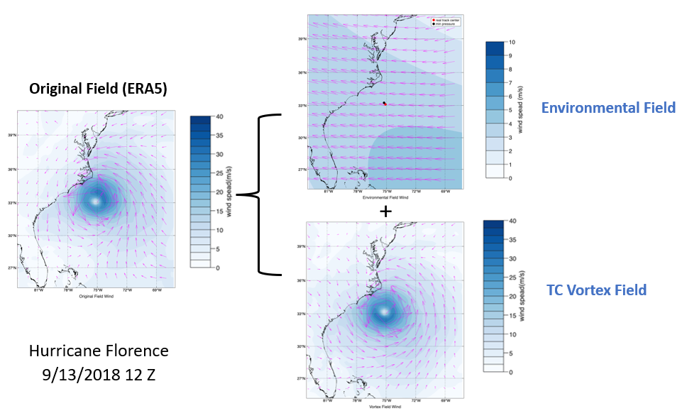
Separated environmental and TC vortex fields from gridded ERA5 for Hurricane Florence.

The separation exists because reanalysis at 0.25° cannot resolve a hurricane’s core: the pressure minimum is too shallow and the maximum winds too weak. Removing the reanalysis vortex and substituting a parametric one preserves the correct large-scale steering flow while restoring a realistic core. See Derivation §4.

The algorithm

Per track time:

1. Read the gridded fields for the time window — getERA5Data.
2. Locate the gridded pressure minimum within search_radius of the track eye — findPressureCenter. This is a diagnostic only; it reports the offset from the track eye.
3. Transform the extraction box to polar coordinates about the eye — convertToPolarCoords.
4. Find three cutlines — findCutline, run three times: once at filter_isotach to set the filter length scale, and once each at wind_threshold_inner and wind_threshold_outer to define the blending masks. Each contour is then smoothed (smoothCutline) and made convex (ensureConvexCutline).
5. Filter — applyButterworthFilter2D / computeBasicField. A 5th-order Butterworth low-pass filter is applied in the zonal and meridional directions, with the half-power length scale set to the mean radius of the filter_isotach contour times filter_hp_multiplier.
6. Store the environmental field, the residual hurricane field, and the two masks — storeResults, then createOutputStruct.

The extraction is centered on the interpolated track eye, not the gridded pressure minimum. findPressureCenter still runs every timestep but only reports the offset between the two as a debug diagnostic. As a consequence the min_pressure_center_lon / min_pressure_center_lat fields in the output struct carry the track position despite their names.

Filter isotach versus blending isotachs

These are independent settings and it is worth being clear about which does what:

Parameter	Controls
filter_isotach, filter_hp_multiplier	The Butterworth half-power length scale — how much energy is assigned to the environmental field
wind_threshold_inner	The inner blending mask, conventionally the 34 kt isotach
wind_threshold_outer	The outer blending mask, conventionally the 20 kt isotach

The inner blending isotach no longer doubles as the filter scale, as it did before v1.5.

Configuration in physical degrees

As of v1.5, SeparateEnvHur is configured in degrees, not numbers of grid cells. The grid increment is detected from the input file at run time as CONFIG.dlonlat — longitude and latitude spacing must be equal — and every cell count is derived from it. The output grid is output_grid_length/dlonlat + 1 points per side. The same configuration therefore works unchanged against input data of any resolution.

Parameter	Meaning	Shipped value
background_file	Gridded NetCDF input, local path or OPeNDAP URL; <year> is substituted at run time	see ERA5 Data
filter_grid_length	Side length (deg) of the box the digital filter runs on	30
output_grid_length	Side length (deg) of the cutline/output box; must be ≤ filter_grid_length	20
search_radius	Radius (deg) searched for the gridded pressure minimum (diagnostic only)	1.5
filter_isotach	Isotach (m/s) whose mean radius sets the filter length scale	17.5
filter_hp_multiplier	Half-power scale = mean radius to filter_isotach × this	25
wind_threshold_inner	Inner blending cutline isotach (m/s)	34 kt
wind_threshold_outer	Outer blending cutline isotach (m/s)	20 kt
num_points_smoother	Moving-mean width for cutline smoothing	3
isotach_smooth_variance	Convergence tolerance for cutline smoothing	2000
num_azimuthal_points	Polar azimuths; taken from GAHM_compute_info.ntheta	24
num_radial_points	Polar radial points; taken from GAHM_compute_info.nr	800
radial_inc	(output_grid_length/2)/num_radial_points	derived
output_file_name	Path (no extension) the .mat is written to; set to env_info.file_name	derived

The fields grid_half_size, output_half_size, filter_domain_size, max_radius_deg, num_azimuth_points, and search_range were removed in v1.5. Full parameter documentation is on the Configuration page.

Running it

The usual path is not to run it at all: run_GAHM2026 invokes it automatically when env_info.type = 3 and the .mat file is missing.

Standalone, with a project configuration file:

cd GAHM2026
addpath('SeparateEnvHur')
env_vals = SeparateEnvHur('config/config_Florence');

Or with a struct built by hand, which also returns the configuration augmented with the values derived from the input file (notably CONFIG.dlonlat and CONFIG.grid_size):

CONFIG = struct('background_file', 'path/to/era5.nc', ...
                'storm_name', 'FLORENCE', 'storm_designation', 'AL06', ...
                'storm_year', 2018, 'track_file', 'input/ibtracs.NA.list.v04r01.csv', ...
                'storm_start', datetime(2018,9,10,0,0,0), ...
                'storm_end', datetime(2018,9,18,0,0,0), ...
                'filter_grid_length', 30, 'output_grid_length', 20, ...
                'search_radius', 1.5, ...
                'wind_threshold_outer', 10, 'wind_threshold_inner', 17.5, ...
                'filter_isotach', 17.5, 'filter_hp_multiplier', 25, ...
                'num_points_smoother', 3, 'isotach_smooth_variance', 2000, ...
                'num_azimuthal_points', 24, 'num_radial_points', 800, ...
                'radial_inc', (20/2)/800, ...
                'output_file_name', 'output/FLORENCE_AL06_2018', ...
                'debug', true);
[env_vals, CONFIG] = SeparateEnvHur(CONFIG);

It can also be handed track data that has already been read, which is how run_GAHM2026 calls it: SeparateEnvHur(sepenvhur, ATCF_data_in).

output_dir, if set, is created but is not joined to output_file_name. This is a known defect carried forward verbatim from v1.5 and recorded in DECISIONS.md; put the directory in output_file_name itself.

Output

The .mat file contains a struct with, for nt times and an nlat × nlon grid:

Field	Dimensions	Contents
Time(i)	nt	datetime
Lo(i,:,:), La(i,:,:)	nt × nlat × nlon	Longitude and latitude grids
env_msl, env_u10, env_v10	nt × nlat × nlon	Environmental pressure (mb) and wind (m/s)
hur_msl, hur_u10, hur_v10	nt × nlat × nlon	Hurricane (residual) pressure and wind
Vortex_mask_outer	nt × nlat × nlon	Outer cutline mask, 0 inside / 1 outside
Vortex_mask_inner	nt × nlat × nlon	Inner cutline mask, 0 inside / 1 outside
distance_outer, distance_inner		Cutline distances
BestTrack_lon(i), BestTrack_lat(i)	nt	Track eye position
min_pressure_center_lon/lat(i)	nt	Also the track eye position — see the note above
units	dictionary	Units metadata

The file must cover every track file time; extra times (hourly, for instance) are fine.

Files written before v1.5 name the outer mask Vortex_mask rather than Vortex_mask_outer. readEnvAndHurrFields2 accepts either, so older .mat files still load.

Plotting the split

addpath('PlotEvalScripts')
obj = GAHM2026Plotter.fromSepEnvHur(env_vals);

obj.contourMap('mvelcon', 1, 5);                        % combined env + hurricane
obj.setOpts('wind', 'clims', [0 16]);
obj.contourMap('velcon', 2, 5, obj.EnvData);            % environmental component only
obj.differenceMap(obj.EnvData, obj.HurData, 'speed', 3, 5);

Requirements

• Signal Processing Toolbox, for designfilt and filtfilt.
• A gridded NetCDF file with u10, v10, msl and a recognizable time axis — see ERA5 Data.
• An IBTrACS, ATCF, or fort.22 track file — see Input Track Files.

Known defects carried forward

Two further defects are preserved verbatim from v1.5 so that regression baselines stay valid. Both are commented at the site and recorded in DECISIONS.md:

• a polar-azimuth misalignment, and
• an uncapped loop in smoothCutline.

Do not silently “fix” either without regenerating baselines.