Examples

1. The Florence matrix
2. Smallest useful runs
3. Other storms
4. Running SeparateEnvHur on its own
5. Blending process
6. Wind adjustment factor (WAF)
7. Plotting results
8. Adding a storm

---

Every example below is a configuration that ships in config/. Run one by passing its name with no path and no extension:

cd GAHM2026
R = run_GAHM2026('config_Florence_envtype3_griddedoutput_WAF');

run_GAHM2026 refuses to overwrite an existing gridded NetCDF. Delete or rename output/<name>.nc between runs of the same configuration.

---

The Florence matrix

Hurricane Florence (2018, AL06) is configured across the three environmental field types, both output types, and with and without the wind adjustment factor. This is the fastest way to see what each switch does, since the storm and time window are held fixed.

Configuration	env_info.type	output_info.type	WAF	Needs ERA5
config_Florence_envtype1_griddedoutput_no_WAF	1	grid	off	no
config_Florence_envtype1_griddedoutput_WAF	1	grid	on	no
config_Florence_envtype1_79pointsoutput_WAF	1	points	on	no
config_Florence_envtype2_griddedoutput_no_WAF	2	grid	off	no
config_Florence_envtype2_griddedoutput_WAF	2	grid	on	no
config_Florence_envtype2_79pointsoutput_WAF	2	points	on	no
config_Florence_envtype3_griddedoutput_no_WAF	3	grid	off	yes
config_Florence_envtype3_griddedoutput_WAF	3	grid	on	yes
config_Florence_envtype3_79pointsoutput_no_WAF	3	points	off	yes
config_Florence_envtype3_79pointsoutput_WAF	3	points	on	yes

What the three environmental types mean:

Type	Environmental field	Varies in
1	ADCIRC/ASWIP: $\lvert V_{env}\rvert = 1.5\,V_{trans}^{0.63}$, with the same radial profile as the vortex gradient wind	time and radius
2	Lin & Chavas (2012) as implemented: $0.6\,V_{trans}$, rotated 20° counterclockwise	time only (spatially constant)
3	Gridded field extracted from ERA5 by SeparateEnvHur	time and space

Types 1 and 2 ignore everything else in env_info and need no reanalysis data — they are the cheap test path. Type 3 pulls ERA5 over OPeNDAP and, if the SeparateEnvHur .mat file is missing, runs the separation first.

The point-output configurations evaluate at 79 lon/lat pairs along the North Carolina coast and sounds rather than on a grid. They return Points_* structs and write no NetCDF. The accompanying WAF file, input/WAF_30deg_10km_6km_15deginc_79points_Florence, is a MAT-file whose point coordinates must match output_info.lon/.lat exactly.

Smallest useful runs

config_Florence_radtest_type{1,2,3}.m cover a three-hour window (2018-09-12 00Z to 03Z) with gridded output and no WAF. Types 1 and 2 finish in seconds and need only the IBTrACS file, which makes them the right first run and the right thing to use when checking that an edit did not break the pipeline.

R = run_GAHM2026('config_Florence_radtest_type1');

Other storms

Configuration	Storm	Notes
config_GAHM2026_default	Florence 2018 (AL06)	The default. env_info.type = 3, gridded output, no WAF, 2018-09-12 to 09-17
config_Florence	Florence 2018 (AL06)	Type 3 from the regional monthly ERA5 file 201809.wna.nc
config_Michael	Michael 2018 (AL14)	Type 3, gridded output
config_Carla_type3	Carla 1961	Type 3 using a global monthly ERA5 file, global.1/uvp/1961/09.nc — the example of a pre-satellite-era storm outside the WNA regional collection

Running SeparateEnvHur on its own

The separation can be run standalone with the same configuration file, which is useful when you want to inspect or plot the environmental/hurricane split before committing to a full GAHM2026 run:

cd GAHM2026
addpath('SeparateEnvHur')
env_vals = SeparateEnvHur('config/config_Florence');

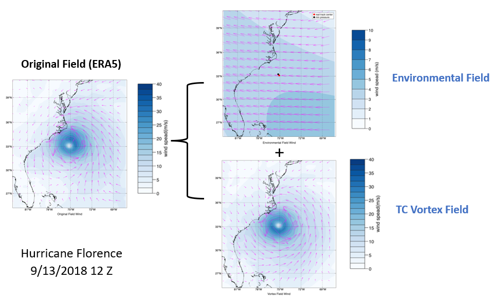
Separated environmental and TC vortex fields from gridded ERA5 for Hurricane Florence.

Blending process

The gridded field is split into an environmental part and a vortex part; the GAHM parametric vortex replaces the ERA5 vortex inside the blending radius; the result is added back to the environmental field.

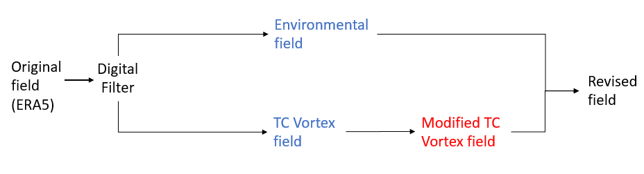
General schematic of the blending strategy.

The taper runs between two radii, controlled by env_info.taper_a, and by convention $r_1$ is the distance to the 34 kt isotach and $r_2$ the distance to the 20 kt isotach:

\[\text{taper} = \tfrac{1}{2}\left(1 + \frac{\tanh\left[a\left(1 - 2\frac{r-r_1}{r_2-r_1}\right)\right]}{\tanh a}\right), \qquad r_1 < r \le r_2\]

with taper $= 1$ inside $r_1$ and $0$ beyond $r_2$. $a = 1$ is nearly linear; $a > 1$ is more S-shaped. env_info.taper_a = 2 is the shipped value.

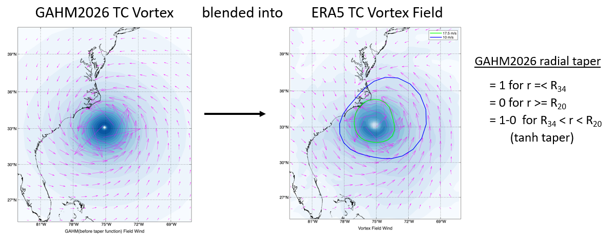
The GAHM2026 vortex to be blended in. Green and blue lines are the 34 kt and 20 kt isotachs.

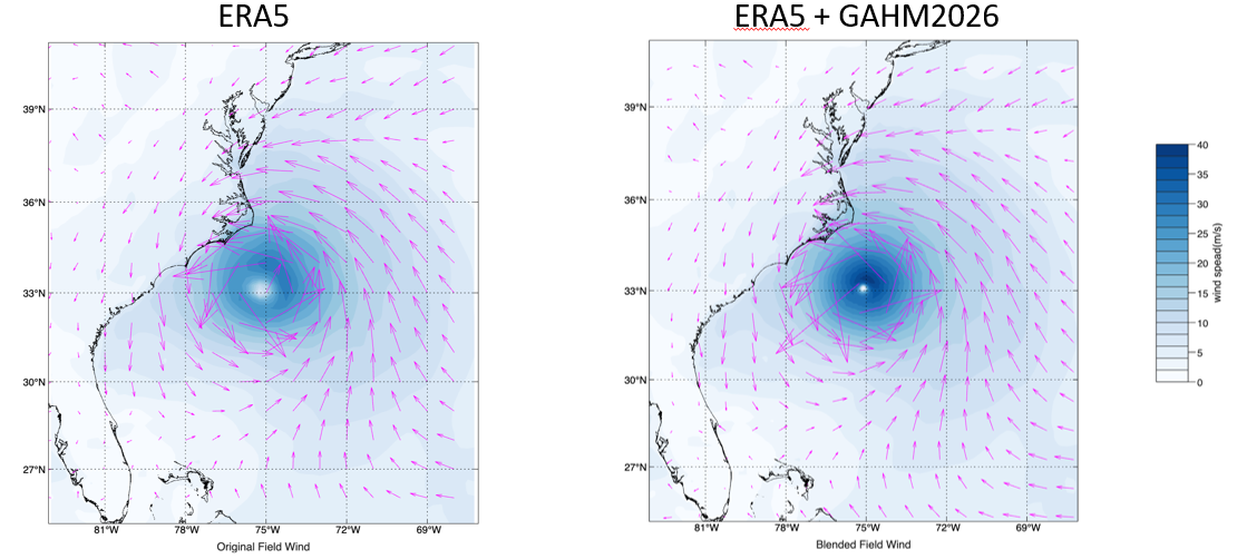
The original ERA5 representation of Florence, and the field after the GAHM2026 vortex is blended in.

See Derivation §4 for the formulation.

Wind adjustment factor (WAF)

Set WAF_info.flag = true and point WAF_info.file_name at a GeoTIFF raster (gridded output) or a MAT-file of precomputed points (point output). The factor is applied to the vortex velocity before the environmental wind is added; pressure is not adjusted.

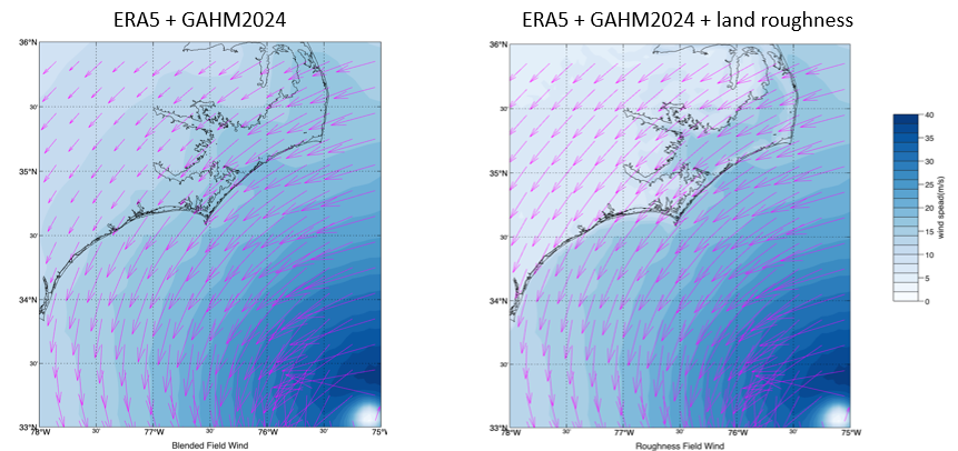
Blended ERA5 + GAHM2026 wind speed with and without WAF. Note the reduction over land and the over-water shadow zones downwind of land.

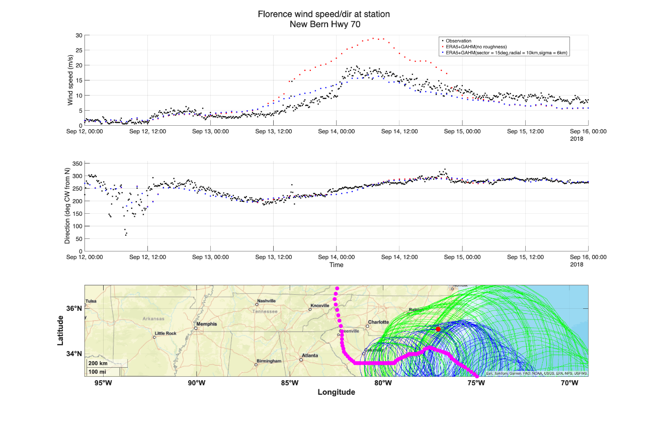
Observations versus blended ERA5 + GAHM2026 wind speed, with and without WAF, at New Bern, NC.

See Derivation §5 for the roughness formulation.

Plotting results

addpath('PlotEvalScripts')
obj = GAHM2026Plotter(R);

fig = obj.contourMap('mvelcon', 1, 20);                        % wind speed map, output time 20
obj.radialProfile('velrad', 'envhur', 10, 10);                 % radial profiles
obj.radialProfile('velrad', {'envhur', 'trackdata'}, 10, 10);  % overlay track data
obj.animate('mvelcon', 1);                                     % GIF / MP4 over all times

From a SeparateEnvHur output struct instead of a GAHM2026 Result:

obj = GAHM2026Plotter.fromSepEnvHur(env_vals);
obj.contourMap('mvelcon', 1, 5);                        % combined env + hurricane
obj.setOpts('wind', 'clims', [0 16]);
obj.contourMap('velcon', 2, 5, obj.EnvData);            % environmental component only
obj.differenceMap(obj.EnvData, obj.HurData, 'speed', 3, 5);

Full method reference on the Plotting page.

Adding a storm

1. Copy the closest existing configuration to config/config_<StormName>.m.
2. Edit the shared identity block — storm_name (all capitals for IBTrACS), storm_year, storm_designation, track_file, and the processing window.
3. Point sepenvhur.background_file at ERA5 data covering the window. See ERA5 Data for the collections and the <year> placeholder.
4. Run it.

The Configuration page documents every parameter you might want to change along the way.